
Introduction
In this article, we will learn how PCA can be used to compress a real-life dataset. We will be working with Labelled Faces in the Wild (LFW), a large scale dataset consisting of 13233 human-face grayscale images, each having a dimension of 64x64. It means that the data for each face is 4096 dimensional (there are 64x64 = 4096 unique values to be stored for each face). We will reduce this dimension requirement, using PCA, to just a few hundred dimensions!
Principal Component Analysis (PCA)
Principal component analysis (PCA) is a technique for reducing the dimensionality of datasets, exploiting the fact that the images in these datasets have something in common. For instance, in a dataset consisting of face photographs, each photograph will have facial features like eyes, nose, mouth. Instead of encoding this information pixel by pixel, we could make a template of each type of these features and then just combine these templates to generate any face in the dataset. In this approach, each template will still be 64x64 = 4096 dimensional, but since we will be reusing these templates (basis functions) to generate each face in the dataset, the number of templates required will be small. PCA does exactly this. Let’s see how!
Dataset
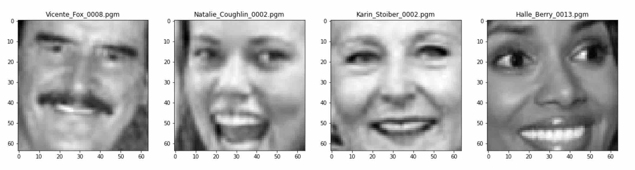
Let’s visualize some images from the dataset. You can see that each image has a complete face, and the facial features like eyes, nose, and lips are clearly visible in each image. Now that we have our dataset ready, let’s compress it.
Compression
PCA is a 4 step process. Starting with a dataset containing n dimensions (requiring n-axes to be represented):
- Step 1: Find a new set of basis functions (naxes) where some axes contribute to most of the variance in the dataset while others contribute very little.
- Step 2: Arrange these axes in the decreasing order of variance contribution.
- Step 3: Now, pick the top k axes to be used and drop the remaining n-k axes.
- Step 4: Now, project the dataset onto these k axes.
These steps are well explained in my previous article. After these 4 steps, the dataset will be compressed from n-dimensions to just k-dimensions (k<n).
Step 1
Finding a new set of basis functions (n-axes), where some axes contribute to most of the variance in the dataset while others contribute very little, is analogous to finding the templates that we will combine later to generate faces in the dataset. A total of 4096 templates, each 4096 dimensional, will be generated. Each face in the dataset can be represented as a linear combination of these templates.

Please note that the scalar constants (k1, k2, …, kn) will be unique for each face.
Step 2
Now, some of these templates contribute significantly to facial reconstruction while others contribute very little. This level of contribution can be quantified as the percentage of variance that each template contributes to the dataset. So, in this step, we will arrange these templates in the decreasing order of variance contribution (most significant…least significant).
Step 3
Now, we will keep the top k templates and drop the remaining. But, how many templates shall we keep? If we keep more templates, our reconstructed images will closely resemble the original images but we will need more storage to store the compressed data. If we keep too few templates, our reconstructed images will look very different from the original images.
The best solution is to fix the percentage of variance that we want to retain in the compressed dataset and use this to determine the value of k (number of templates to keep). If we do the math, we find that to retain 99% of the variance, we need only the top 577 templates. We will save these values in an array and drop the remaining templates.
Let’s visualize some of these selected templates.
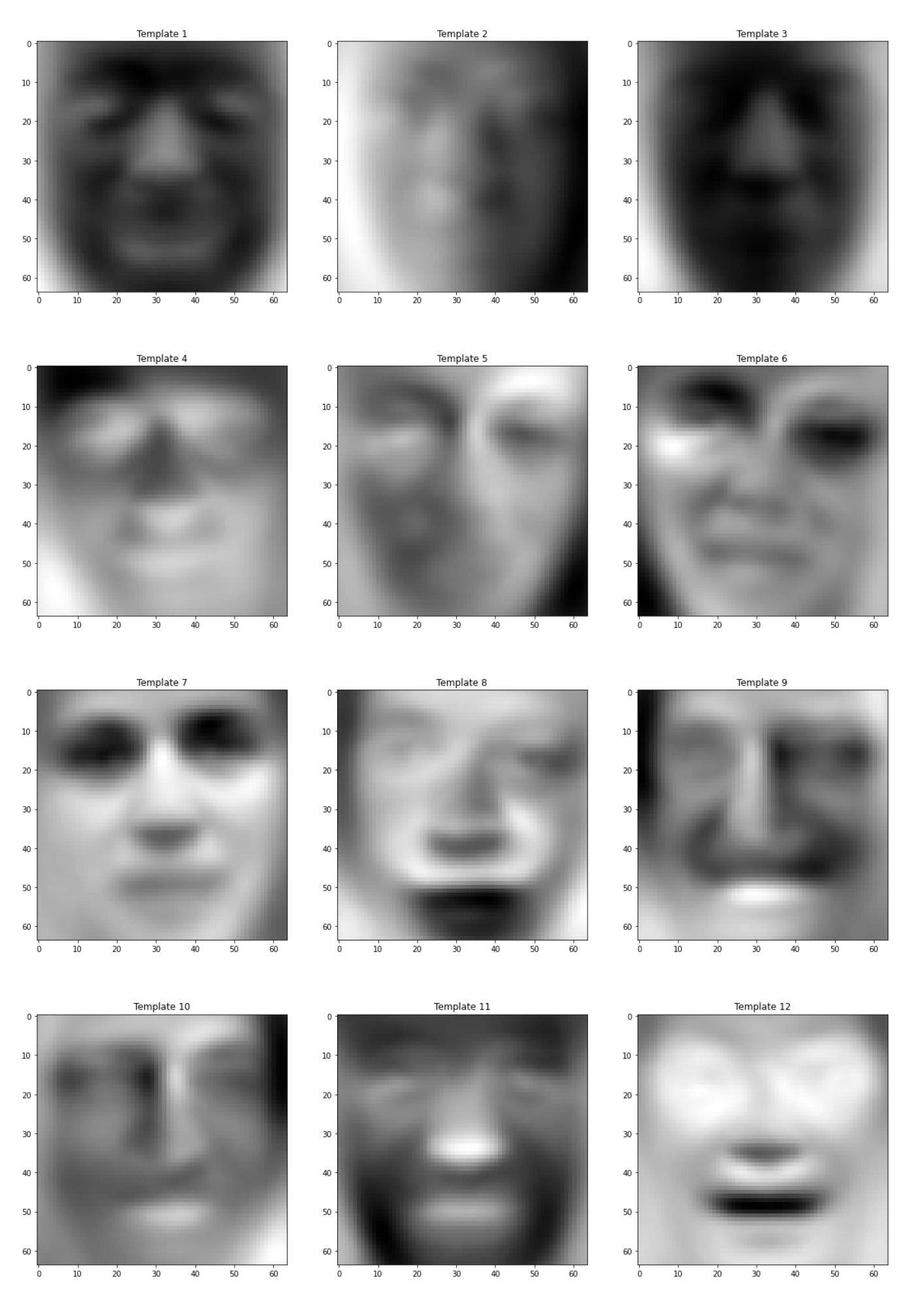
Please note that each of these templates looks somewhat like a face. These are called as Eigenfaces.
Step 4
Now, we will construct a projection matrix to project the images from the original 4096 dimensions to just 577 dimensions. The projection matrix will have a shape (4096, 577), where the templates will be the columns of the matrix.
Before we go ahead and compress the images, let’s take a moment to understand what we really mean by compression. Recall that the faces can be generated by a linear combination of the selected templates. As each face is unique, every face in the dataset will require a different set of constants (k1, k2, …, kn) for the linear combination.
Let’s start with an image from the dataset and compute the constants (k1, k2, …, kn), where n = 577. These constants along with the selected 577 templates can be plugged in the equation above to reconstruct the face. This means that we only need to compute and save these 577 constants for each image. Instead of doing this image by image, we can use matrices to compute these constants for each image in the dataset at the same time.
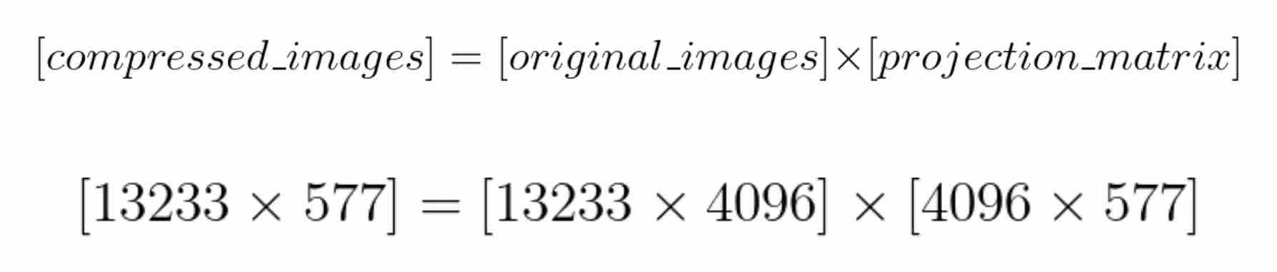
Recall that there are 13233 images in the dataset. The matrix compressed_images contains the 577 constants for each image in the dataset. We can now say that we have compressed our images from 4096 dimensions to just 577 dimensions while retaining 99% of the information.
Compression Ratio
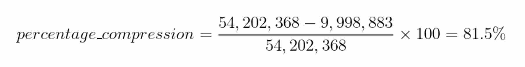
Let’s calculate how much we have compressed the dataset. Recall that there are 13233 images in the dataset and each image is 64x64 dimensional. So, the total number of unique values required to store the original dataset is13233 x 64 x 64 = 54,202,368 unique values.
After compression, we store 577 constants for each image. So, the total number of unique values required to store the compressed dataset is13233 x 577 = 7,635,441 unique values. But, we also need to store the templates to reconstruct the images later. Therefore, we also need to store577 x 64 x 64 = 2,363,392 unique values for the templates. Therefore, the total number of unique values required to store the compressed dataset is7,635,441 + 2,363,392 = 9,998,883 unique values.
We can calculate the percentage compression as:
Reconstruct the Images
The compressed images are just arrays of length 577 and can’t be visualized as such. We need to reconstruct it back to 4096 dimensions to view it as an array of shape (64x64). Recall that each template has a dimension of 64x64 and that each constant is a scalar value. We can use the equation below to reconstruct any face in the dataset.
Again, instead of doing this image by image, we can use matrices to reconstruct the whole dataset at once, with of course a loss of 1% variance.

Let’s look at some reconstructed faces.
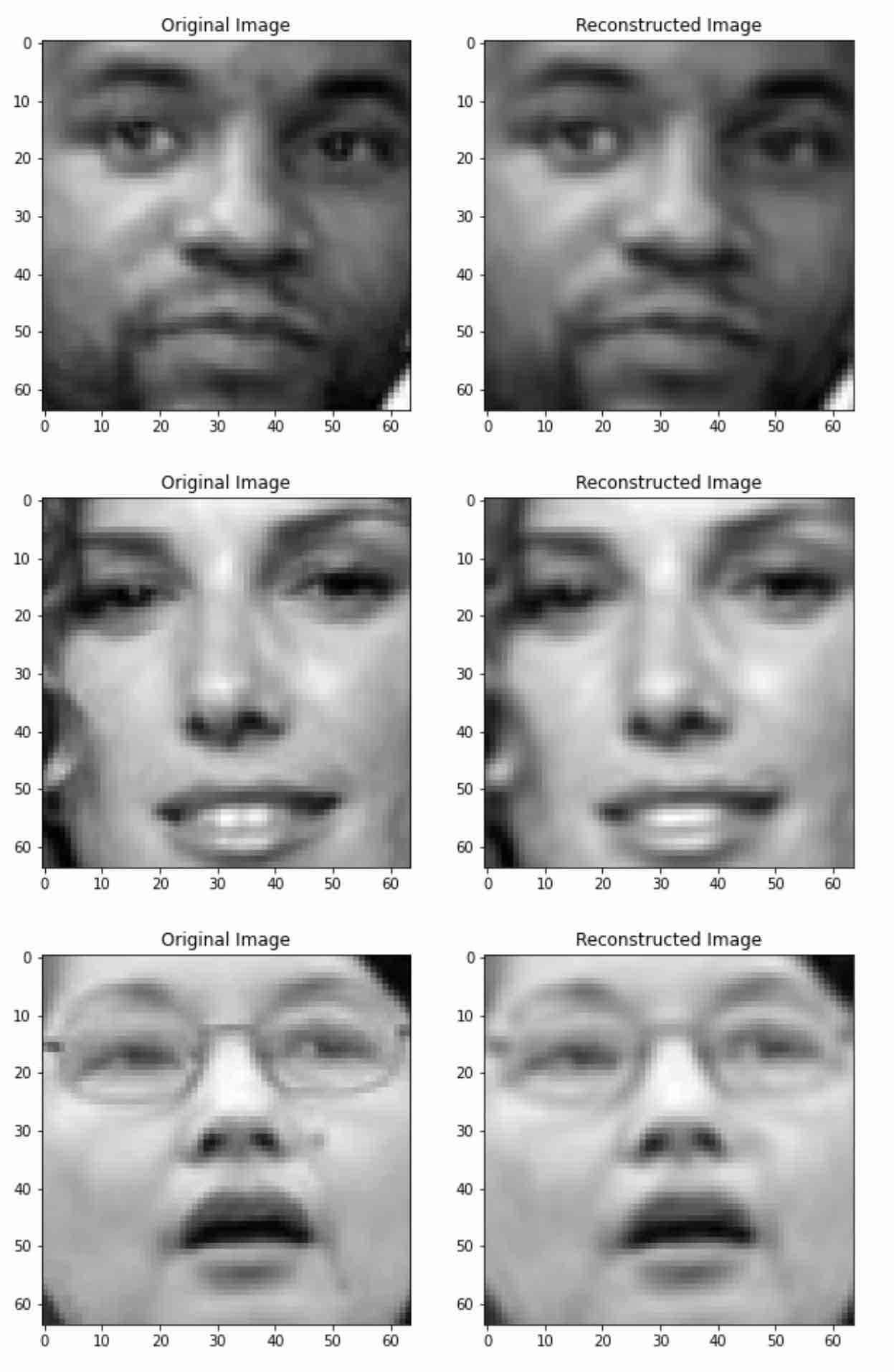
We can see that the reconstructed images have captured most of the relevant information about the faces and the unnecessary details have been ignored. This is an added advantage of data compression, it allows us to filter unnecessary details (and even noise) present in the data.
That’s all folks!
If you made it till here, hats off to you! In this article, we learnt how PCA can be used to compress Labelled Faces in the Wild (LFW), a large scale dataset consisting of 13233 human-face images, each having a dimension of 64x64. We compressed this dataset by over 80% while retaining 99% of the information.
Colab Notebook
View my Colab Notebook for a well commented code!