
Introduction to machine learning
In the traditional hard-coded approach, we program a computer to perform a certain task. We tell it exactly what to do when it receives a certain input. In mathematical terms, this is like saying that we write the f(x) such that when users feed the input x into f(x), it gives the correct output y.
 In machine learning, however, we have a large set of inputs x and corresponding outputs y but not the function f(x). The goal here is to find the f(x) that transforms the input x into the output y. Well, that’s not an easy job. In this article, we will learn how this happens.
Dataset
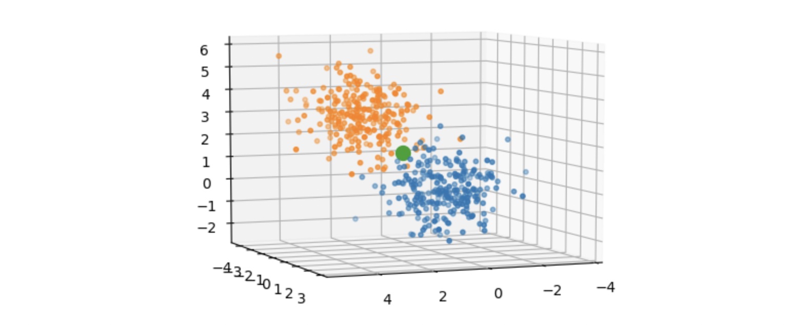
To visualize the dataset, let’s make our synthetic dataset where each data point (input x) is 3 dimensional, making it suitable to be plotted on a 3D chart. We will generate 250 points (cluster 0) in a cluster centered at the origin (0, 0, 0). A similar cluster of 250 points (cluster 1) is generated but not centered at the origin. Both clusters are relatively close but there is a clear separation as seen in the image below. These two clusters are the two classes of data points. The big green dot represents the centroid of the whole dataset.
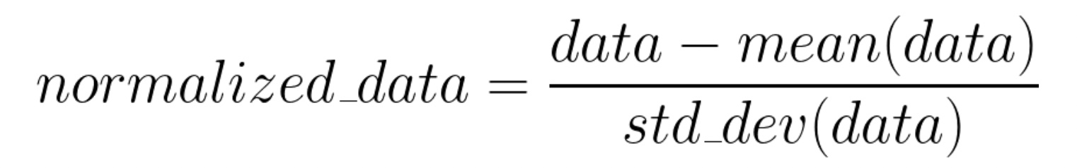
After generating the dataset, we will normalize it by subtracting the mean and dividing by the standard deviation. This is done to zero-center the data and map values in each dimension in the dataset to a common scale. This speeds up the learning.
The data will be saved in an array X containing the 3D coordinates of normalized points. We will also generate an array Y with the value either 0 or 1 at each index depending on which cluster the 3D point belongs.
Learnable Function
Now that we have our data ready, we can say that we have the x and y. We know that the dataset is linearly separable implying that there is a plane that can divide the dataset into the two clusters, but we don’t know what the equation of such an optimal plane is. For now, let’s just take a random plane.
The function f(x) should take a 3D coordinate as input and output a number between 0 and 1. If this number is less than 0.5, this point belongs to cluster 0 otherwise, it belongs to cluster 1. Let’s define a simple function for this task.

x: input tensor of shape (num_points, 3)W: Weight (parameter) of shape (3, 1) chosen randomlyB: Bias (parameter) of shape (1, 1) chosen randomlySigmoid: A function that maps values between 0 and 1
Let’s take a moment to understand what this function means. Before applying the sigmoid function, we are simply creating a linear mapping from the 3D coordinate (input) to 1D output. Therefore, this function will squish the whole 3D space onto a line meaning that each point in the original 3D space will now be lying somewhere on this line. Since this line will extend to infinity, we map it to [0, 1] using the Sigmoid function. As a result, for each given input, f(x) will output a value between 0 and 1.
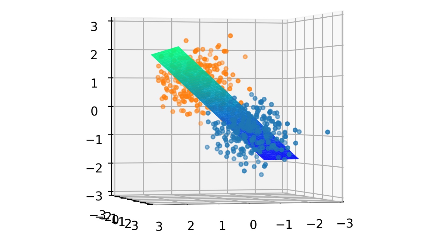
Remember that W and B are chosen randomly and so the 3D space will be squished onto a random line. The decision boundary for this transformation is the set of points that make f(x) = 0.5. Think why! As the 3D space is being squished onto a 1D line, a whole plane is mapped to the value 0.5 on the line. This plane is the decision boundary for f(x). Ideally, it should divide the dataset into two clusters but since W and B are randomly chosen, this plane is randomly oriented as shown below.
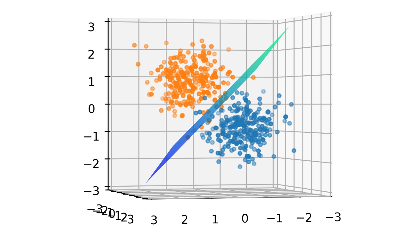
Our goal is to find the right values for W and B that orients this plane (decision boundary) in such a way that it divides the dataset into the two clusters. This when done, yields a plane as shown below.
Loss
So, we are now at the starting point (random decision boundary) and we have defined the goal. We need a metric to decide how far we are from the goal. The output of the classifier is a tensor of shape (num_points, 1) where each value is between [0, 1]. If you think carefully, these values are just the probabilities of the points belonging to cluster 1. So, we can say that:
- f(x) = P(x belongs to cluster 1)
- 1-f(x) = P(x belongs to cluster 0)
It wouldn’t be wrong to say that [1-f(x), f(x)] forms a probability distribution over the clusters 0 and cluster 1 respectively. This is the predicted probability distribution. We know for sure which cluster every point in the dataset belongs to (from y). So, we also have the true probability distribution as:
- [0, 1] when x belongs to the cluster 1
- [1, 0] when x belongs to the cluster 0
A good metric to calculate the incongruity between two probability distributions is the Cross-Entropy function. As we are dealing with just 2 classes, we can use Binary Cross-Entropy (BCE). This function is available in PyTorch’s torch.nn module. If the predicted probability distribution is very similar to the true probability distribution, this function returns a small value and vice versa. We can average this value for all the data points and use it as a parameter to test how the classifier is performing.
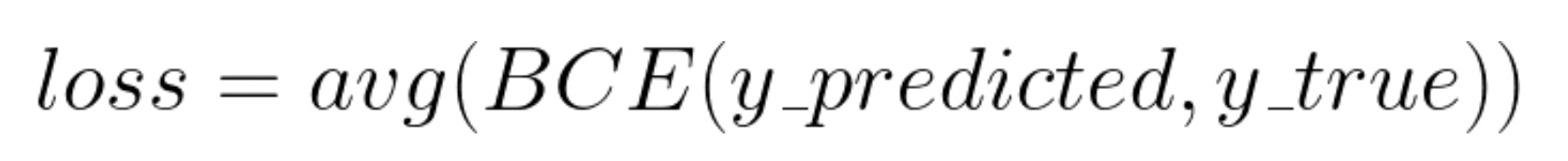
This value is called the loss and mathematically, our goal now is to minimize this loss.
Training
Now that we have defined our goal mathematically, how do we reach our goal practically? In other words, how do we find optimal values for W and B? To understand this, we will take a look at some basic calculus. Recall that we currently have random values for W and B. The process of learning or training or reaching the goal or minimizing the loss can be divided into two steps:
- Forward-propagation: We feed the dataset through the classifier f(x) and use BCE to find the loss.
- Backpropagation: Using the loss, adjust the values of W and B to minimize the loss.
The above two steps will be repeated over and over again until the loss stops decreasing. In this condition, we say that we have reached the goal!
Backpropagation
Forward propagation is simple and already discussed above. However, it is essential to take a moment to understand backpropagation as it is the key to machine learning. Recall that we have 3 parameters (variables) in W and 1 in B. So, in total, we have 4 values to optimize.

Once we have the loss from forward-propagation, we will calculate the gradients of the loss function with respect to each variable in the classifier. If we plot the loss for different values of each parameter, we can see that the loss is minimum at a particular value for each parameter. I have plotted the loss vs parameter for each parameter.
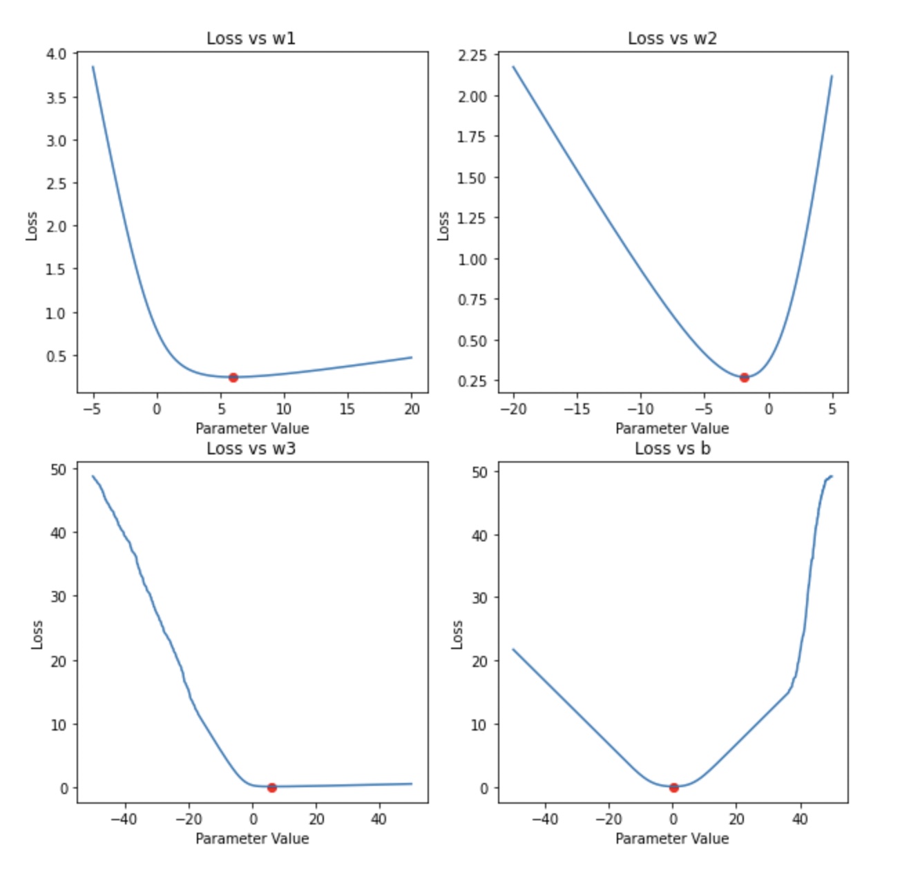
An important observation to make here is that the loss is minimized at a particular value for each of these parameters as shown by the red dot.
Let’s consider the first plot and discuss how w1 will be optimized. The process remains the same for the other parameters. Initially, the values for W and B are chosen randomly and so (w1, loss) will be randomly placed on this curve as shown by the green dot.
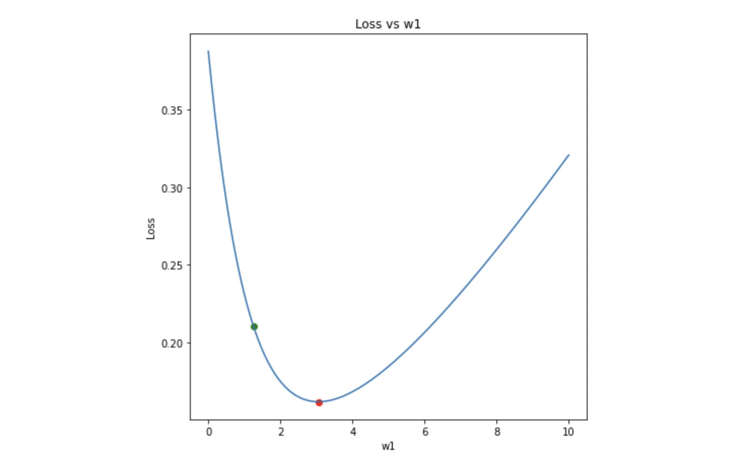
Now, the goal is to reach the red dot, starting from the green dot. In other words, we need to move downhill. Looking at the slope of the curve at the green dot, we can tell that increasing w1 (moving right) will lower the loss and therefore move the green dot closer to the red one. In mathematical terms, if the gradient of the loss with respect to w1 is negative, increase w1 to move downhill and vice versa. Therefore, w1 should be updated as:
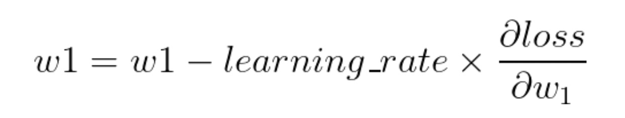
The equation above is known as gradient descent equation. Here, the learning_rate controls how much we want to increase or decrease w1. If the learning_rate is large, the update will be large. This could lead to w1 going past the red dot and therefore missing the optimal value. If this value is too small, it will take forever for w1 to reach the red dot. You can try experimenting with different values of learning rate to see which works the best. In general, small values like 0.01 works well for most cases.
In most cases, a single update is not enough to optimize these parameters; so, the process of forward-propagation and backpropagation is repeated in a loop until the loss stops reducing further. Let’s see this in action:

An important observation to make is that initially the green dot moves quickly and slows down as it gradually approaches the minima. The large slope (gradient) during the first few epochs (when the green dot is far from the minima) is responsible for this large update to the parameters. The gradient decreases as the green dot approaches the minima and thus the update becomes slow. The other three parameters are trained in parallel in the exact same way. Another important observation is that the shape of the curve changes with epoch. This is due to the fact that the other three parameters (w2, w3, b) are also being updated in parallel and each parameter contributes to the shape of the loss curve.
Visualize
Let’s see how the decision boundary updates in real-time as the parameters are being updated.

That’s all folks!
If you made it till here, hats off to you! In this article, we took a visual approach to understand how machine learning works. So far, we have seen how a simple 3D to 1D mapping, f(x), can be used to fit a decision boundary (2D plane) to a linearly separable dataset (3D). We discussed how forward propagation is used to calculate the loss followed by backpropagation where gradients of the loss with respect to parameters are calculated and the parameters are updated repeatedly in a training loop.